Understanding Megatron-Style Tensor Parallelism

27 May, 2025

Last updated 2 months, 4 weeks

Transformers are known to be extremely effective at scaling up and being trained in parallel. This feature is why the current Deep Learning revolution started in 2019 with things like the GPT series of models which used hundreds of GPUs to train models that were larger than anything before it.

In those days, the most popular method of distributed training was called the Distributed Data Parallelism (DDP). DDP basically creates a copy of the model in every GPU available and then synchronises the data loader in such a way that each copy of the model receives a fresh set of data that the others don’t have.

In this way, the model could calculate the gradient updates on humongous batches across the GPU’s and then synchronise the gradients across them to apply updates to the model weights.

The problem with DDP however, is that the VRAM inside a GPU was the limiting factor for the models, since they could only get so big before they fill up the entire GPU’s memory.

GEMMs, or General Matrix Multiplications are simple matrix multiplications that are are ever present in neural networks. Most of the transformer architecture is made up of GEMM operations and it is this key fact that allows transformer models to be scaled to hundreds of billions of parameters across hundreds of thousands of GPU’s during training.

Exploring the GEMM

Let’s consider the input tensor to a feedforward layer, ignoring (squeezing) the batch dimension and taking the transpose of the sequence length $seq\_len$ and embedding dimension $d_{h i d d e n}$ so that the input shape is $(seq\_len, d_{h i d d e n})$ .

Suppose the input tensor is a sequence of 3 tokens with a hidden dimension of 2 for each token.

x = [\begin{matrix} 1 & 2 \\ 2 & 8 \\ 2 & 3 \end{matrix}]

In practise the number of tokens (number of rows) will vary for each sequence in the batch but that isn’t important for our exercise since the left matrix multiplication doesn’t require the items in the $0^{t h}$ to be a specific size.

Next suppose we have a projection matrix $W_{u p}$ which takes each of the tokens in the sequence and projects it up to $4 \times d_{h i d d e n}$ .

W_{u p} = [\begin{matrix} 1 & 0 & 2 & 1 & 0 & 3 & 1 & 4 \\ 2 & 1 & 0 & 2 & 3 & 0 & 2 & 1 \end{matrix}]

These two matrices will be multiplied as $x W_{u p}$ to produce the below projected tensor.

Y = [\begin{matrix} 1 & 2 \\ 2 & 8 \\ 2 & 3 \end{matrix}] [\begin{matrix} 1 & 0 & 2 & 1 & 0 & 3 & 1 & 4 \\ 2 & 1 & 0 & 2 & 3 & 0 & 2 & 1 \end{matrix}] = [\begin{matrix} 4 & 2 & 2 & 5 & 6 & 3 & 5 & 6 \\ 18 & 8 & 4 & 18 & 24 & 8 & 18 & 16 \\ 8 & 3 & 4 & 8 & 9 & 6 & 8 & 11 \end{matrix}]

This new representation of the input matrix has the embedding dimensions projected up to $4 \times d_{h i d d e n}$ , allowing for the network to perform some computation on the tokens with the added parameters.

This projected activation must then have a non-linearity, let’s say the GeLU operator in our example. For simplicity, lets pretend the GeLU operator is just an Identity matrix and doesn’t change anything (it’s gonna make life painful to prove an idea later if we do otherwise).

After we perform the non-linear GeLU function to this Y, we will GEMM it with a projection down matrix which will take it back down to $d_{h i d d e n}$ .

W_{d o w n} = [\begin{matrix} 1 & 2 \\ 0 & 1 \\ 2 & 0 \\ 1 & 2 \\ 0 & 3 \\ 3 & 0 \\ 1 & 2 \\ 4 & 1 \end{matrix}]

And we can see then that the final output $O$ of the feedforward is below.

O = Y W_{d o w n} = [\begin{matrix} 51 & 54 \\ 150 & 204 \\ 94 & 89 \end{matrix}]

General Matrix Multiplication

The General Matrix Multiplication (GEMM) is the fundamental operation that is performed at every single part of the transformer. It is present in everything from the embedding to the QKV operations to the final language modelling head in a transformer.

GPU’s are extremely efficient at calculating GEMMs due to specialised hardware design which has cores that are specifically designed to perform the matrix multiplications extremely fast.

The problem with scaling up the transformer models however, is that the GEMMs can become extremely large within the model. Some of the mid-sized open source models today have around 8,192 dimensional embeddings and context lengths up to 200k. This means that when projecting up to $4 \times 8, 192 = 32, 769$ , our feedforward would need to store around $8, 192 \times 32, 769 = 268, 435, 456$ parameters in just a single GPU.

This doesn’t even include the projection down operator right after, which adds the same number of parameters again. In half precision training, this can take over 1 GB for just this one single feedforward layer in one single block of the training (there’s usually around 80 blocks with these for 70B LLM’s).

So how then can we split matrix operations this big across multiple GPU’s without introducing catastrophic communication latency in training?

Megatron-LM: Invention of Tensor Parallelism

In 2020 labs such as OpenAI had already been developing internal systems to perform massively parallel training of massive models, but the open source world was still pretty far behind. Only a few players like Meta and Google had any experience in maintaining huge AI systems at scale. This was still the early days before ChatGPT and the rest of the craze had come into vogue.

It was at this time that Nvidia released a paper titled “Megatron-LM: Training Multi-Billion Parameter Language Models Using Model Parallelism”. This paper introduced a novel training system that focused not on Data Parallelism, but tensor parallelism instead.

The idea of Tensor Parallelism is basically that we can take the parameters of the feedforward layer, and “shard” them across multiple GPU’s so that each GPU only holds a fraction of the weights. For the remainder of this explanation, let’s say we are only splitting it across 2 GPU’s

Tensor Parallelising the FeedForward layers

Recall the feedforward example from before with the input tensor to a feedforward layer, has shape $(seq\_len, d_{h i d d e n})$ . Let’s consider the same tensor from which has a sequence length of 3 tokens with a hidden dimension of 2 for each token.

x = [\begin{matrix} 1 & 2 \\ 2 & 8 \\ 2 & 3 \end{matrix}]

Let’s bring back the same weight projection matrix will use the same projection matrix $W_{u p}$ which takes each of the tokens in the sequence and projects it up to $4 \times d_{h i d d e n}$ .

W_{u p} = [\begin{matrix} 1 & 0 & 2 & 1 & 0 & 3 & 1 & 4 \\ 2 & 1 & 0 & 2 & 3 & 0 & 2 & 1 \end{matrix}]

Now applying the idea for Tensor Parallelism, we will shard this into two seperate matrices

W_{u p}^{1} = [\begin{matrix} 1 & 0 & 2 & 1 \\ 2 & 1 & 0 & 2 \end{matrix}], W_{u p} = [\begin{matrix} 0 & 3 & 1 & 4 \\ 3 & 0 & 2 & 1 \end{matrix}]

These two sharded matrices can then be sent to two seperate GPU’s, where they will each receive the same input tensor to then each produce a sharded tensor output $Y^{i}$ .

In GPU#1:

Y^{1} = [\begin{matrix} 1 & 2 \\ 2 & 8 \\ 2 & 3 \end{matrix}] [\begin{matrix} 1 & 0 & 2 & 1 \\ 2 & 1 & 0 & 2 \end{matrix}] = [\begin{matrix} 4 & 2 & 2 & 5 \\ 18 & 8 & 4 & 18 \\ 8 & 3 & 4 & 8 \end{matrix}]

In GPU#2:

Y^{2} = [\begin{matrix} 1 & 2 \\ 2 & 8 \\ 2 & 3 \end{matrix}] [\begin{matrix} 0 & 3 & 1 & 4 \\ 3 & 0 & 2 & 1 \end{matrix}] = [\begin{matrix} 6 & 3 & 5 & 6 \\ 24 & 8 & 18 & 16 \\ 9 & 6 & 8 & 11 \end{matrix}]

If you compare to the full output that we calculated before, you will notice that this output is simply the two sharded matrices joined along column-wise, the same way they had been split. That is to say $Y = [Y^{1}, Y^{2}]$

Now we have to apply a non-linearity like GeLU at this stage for the feedforward layer, but recall that we said earlier that for our example, we can just pretend that the GeLU non-linearity is just the identity operation. We did this because we don’t want to prove the following results, but the identity operation is self explanatory and also satisfies it.

In the Megatron LM, we don’t need to join the sharded activations $Y^{1}$ or $Y^{2}$ yet because we can take advantage of the fact that the GELU operator in the feed forward layer satisfies the property $G e L U (X A) = G e L U (X A^{1}) + G e l u (X A^{2})$ as long as the sharded matrix A is split column-wise.

This means we can keep going with our model in this sharded state and complete the GeLU operation without needing an all-reduce to make all the GPU’s have the same stuff yet.

After the GeLU activation function, we will need to project our two matrices back down to $d_{h i d d e n}$ with another projection matrix $W_{d o w n}$ .

W_{d o w n} = [\begin{matrix} 1 & 2 \\ 0 & 1 \\ 2 & 0 \\ 1 & 2 \\ 0 & 3 \\ 3 & 0 \\ 1 & 2 \\ 4 & 1 \end{matrix}]

It can be seen here that since the sharding was applied column-wise before, the resulting outputs $Y^{i}$ are also sharded column-wise. This means that the next proceeding operation will need to sharded row wise in order to make all the dimensions match up. Our sharded down projection matrix will be the below two matrices.

W_{d o w n}^{1} = [\begin{matrix} 1 & 2 \\ 0 & 1 \\ 2 & 0 \\ 1 & 2 \end{matrix}], W_{d o w n}^{2} = [\begin{matrix} 0 & 3 \\ 3 & 0 \\ 1 & 2 \\ 4 & 1 \end{matrix}]

These sharded projections can then be applied to the sharded outputs of the GeLU layer to produce the final outputs.

O^{1} = [\begin{matrix} 4 & 2 & 2 & 5 \\ 18 & 8 & 4 & 18 \\ 8 & 3 & 4 & 8 \end{matrix}] [\begin{matrix} 1 & 2 \\ 0 & 1 \\ 2 & 0 \\ 1 & 2 \end{matrix}], O^{2} = [\begin{matrix} 6 & 3 & 5 & 6 \\ 24 & 8 & 18 & 16 \\ 9 & 6 & 8 & 11 \end{matrix}] [\begin{matrix} 0 & 3 \\ 3 & 0 \\ 1 & 2 \\ 4 & 1 \end{matrix}]

Which produce the following two shards:

O^{1} = [\begin{matrix} 13 & 20 \\ 44 & 80 \\ 24 & 35 \end{matrix}], O^{2} = [\begin{matrix} 38 & 34 \\ 106 & 124 \\ 70 & 54 \end{matrix}] .

The keen eye will notice that the two shards above can simply be added together to produce the original output $O$ that we had produced.

This is where our first All-Reduce operation finally comes in, since we will need to make sure that this final output is the same as the un-sharded result prior to being added to the residual stream and also prior to being passed through the dropout layer during the training phase.

Tensor Parallelising the Attention layers

The attention layer is already pretty parallelisable due to the attention heads. The layer can be split by these attention heads so that each rank in a node will have it’s own set of attention heads. This will create a set of Sharded output heads.

The attention layer can also be parallelised by splitting each Q and K matrix by rows and columns respectively. The operations all work out to be separable since it can be thought of as basically processing

These heads in a regular MHA layer are concatenated but in this case, we will let the sharded parts complete a computation of the output projection that is sharded $Y_{i} W_{i}^{O}$ .

The reason this is possible is because we will split the Output projection matrix along its sequence dimension since the MHA heads are each produced by splitting along the embedding dimension of the input. This means that the Output projection matrix will still produce activations of the same dimension (projects the head dimension up to the hidden dimension), albeit only a partial amount of it.

This partial amount must then be summed using all-reduce across the GPU’s in order to create the final full output that can be added to the residual stream with the same shape and output as an unsharded full operation.

Benefits

Allows training of much larger models in memory constrained GPU’s and clusters of memory constrained GPU’s
Reduces the size of the activations at the large MatMul’s by splitting them across the local node. We project the dimensions up super duper high so the peak activation memory at this stage would be enormous on a single GPU. Read my memory blog post to understand why
TP is actually better for inference because its memory reductions allow for larger KV-cache sizes, which can greatly improve efficiency.
Tensor parallelism is particularly well-suited to inference architecturally, because only the activations are communicated around (unlike FSDP/ZeRO3, which would communicate weights for every newly-generated token) and every rank is involved in every step of the computation (unlike Pipeline parallelism, in which GPUs would necessarily idle) ¹

Problems

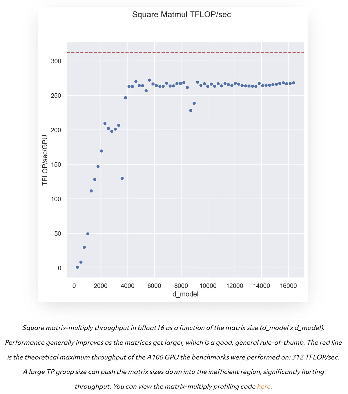
Modern GPU’s actually prefer larger MatMuls- Despite achieving the goal of splitting MatMuls, modern GPU’s are actually shown to perform progressively better on larger matrix multiplications. This is because larger matrix multiplications are able to leverage more of the TFLOPs of compute available on the more powerful GPU’s today.
- Throughput vs Model size in an A100 GPU
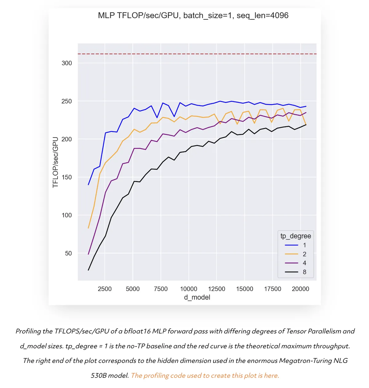
- Throughput vs Model size in an A100 GPU with varying TP degree
Slows Down the Forward Pass- The parallelism requires an All-Reduce operation at every output layer, which adds too much communication latency to models. As we mentioned before, the communication in training is more expensive than the computation since the computation is performed more efficiently.
High Activation Memory from Re-computations- The Dropout and Layer Norm operations are identically calculated on multiple GPU’s while shared in the original paper. While this traded more computation for less communication overhead, it did multiply Activation Memory when it passed through these layers. This was later tackled in a paper that parallelised these layers at the sequence dimension ².

#AI