Understanding KL Divergence in Reinforcement Learning

18 Apr, 2025

Last updated 4 months

The Kullback-Leibler Divergence (KL) divergence is a way to measure how much one distribution diverges from another. This is used in Machine Learning frequently when a new network, $Q(x)$, is being optimised without diverging too far from a reference network, $P(x)$.

The regular KL divergence, known as the forward KL divergence, exhibits a “mean-seeking” behaviour, which introduces an important consideration when tackling optimisation problems. This mean seeking behaviour is best demonstrated in distributions which have multiple modes.

The $Q(x)$ distribution when optimised for minimal KL divergence in such cases tends towards a position that maximises the amount of the $Q(x)$ distribution that is captured in the area under $P(x)$. This is because the importance of the penalty in a region is weighted by $P(x)$ and wherever it is highest.

Studying the Forward Kullback-Leibler Divergence

The forward KL divergence has the formula

where the value that is produced represents the divergence of P from Q. This is the difference between the two distributions weighted by $P(x)$ .

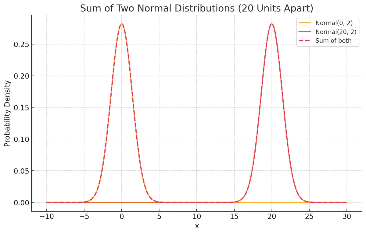
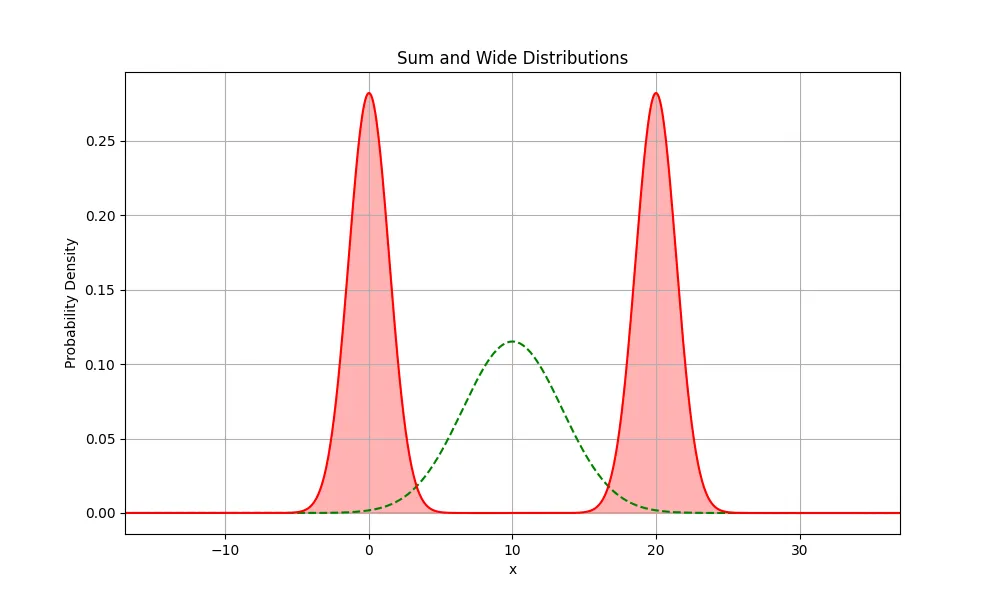
Let’s consider a probability distribution with multiple modes such as a function that is a sum of two univariate Normal distributions. This may look like the following graph with the equation $P(x)=N(\mu =0,\sigma =2)+N(\mu =20,\sigma =2)$.

Now suppose we have another distribution $Q(x)$, which we initialise with a random mean and variance of $\mu =5$ and ${\sigma }^2=5$.

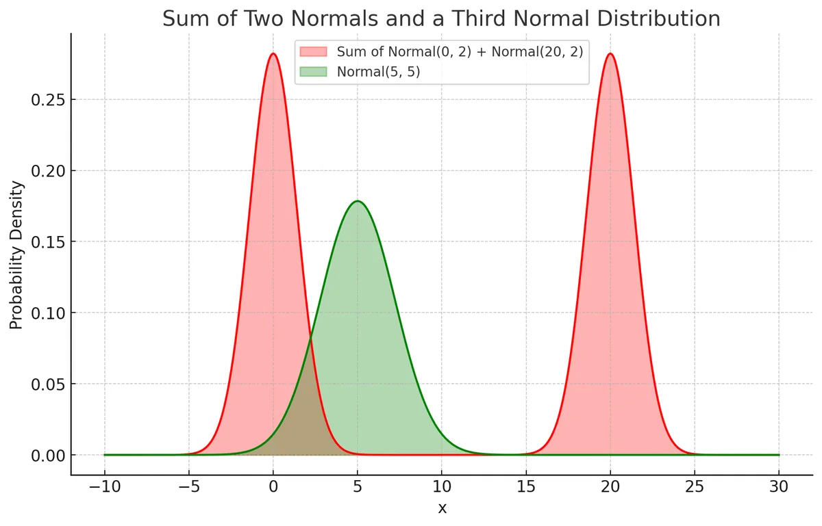
What would happen if we tried to optimise this new distribution $Q(x)$ according to the forward KL divergence it displays from the target distribution.

There are basically 3 main zones for where this $Q(x)$ can go on this graph.

1. To the far left or far right, beyond the distribution modes
2. To the immediate left or right , under either of the distribution mode
3. Stay near the centre

Let’s explore each.

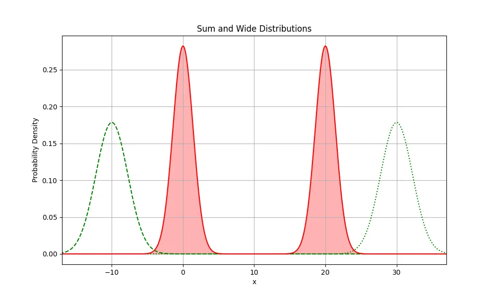
Far left or far right

At these positions, the KL divergence would be extremely high because the weighting of the divergence is most strongly influenced by the peaks of the parent distribution. This is true regardless of which direction the $Q(x)$ is moved (dashed and dotted lines)

Far away on either side makes the distribution have a high KL penalty, where the importance of a low penalty are the highest but the value $log(P(x))-log(Q(x))$ is extremely high. The $log(P(x))$ can be seen to be very high at the points where the $Q(x)$ is 0. Super high penalty!

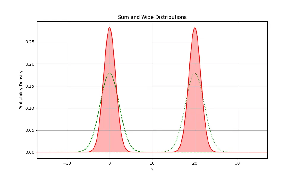
Immediate left or right

At these positions, the $Q(x)$ will have a much lower penalty than being on either of the extremes. Regardless of whichever mode it picks to sit under however, it will get highly penalised for missing the other mode severely, once again due to the weighting factor in front of the divergence term $log(P(x))-log(Q(x))$.

Centre

At this position, the penalty is the lowest since it can cover as much of both of the highest weighted areas of the graphs. The distribution will spread out to cover as much area as possible between the two modes. This has much lower penalty than either of the other two options above.

Analysis of behaviour

Notice how the distribution expanded in variance and aligned itself to sit in between the two modes, not particularly imitating wither of the modes? The $Q(x)$ when optimised on the forward KL will seek to towards a mean, regardless of where it is initially located.

This can be problematic if your goal is to restrict the variance of a distribution and to only mildly wiggle the $Q(x)$ distribution around the target distribution.

In Reinforcement Learning, models are typically optimised to maximise an objective function that looks like something like the below equation.

Here the reward objective can be thought to represent some implicit distribution (it's inferred from the rewards and there's no distribution it can just copy) for the model to update it weights to maximise. The updates to the parameters if too large however, can cause instability in training. Due to this, the model is usually grounded in some reference models distribution to ensure that the updates are penalised for being too large, usually using the KL divergence.

In our context, this looks like the sum of two distributions that we began this post with. The reference distribution will basically be the $P(x)$ we try to stay near, while the divergence of our models predictions, $Q(x)$, will be penalised for diverging too far.

An example of how $Q(x)$ and $P(x)$ might look initially in such a case is displayed below.

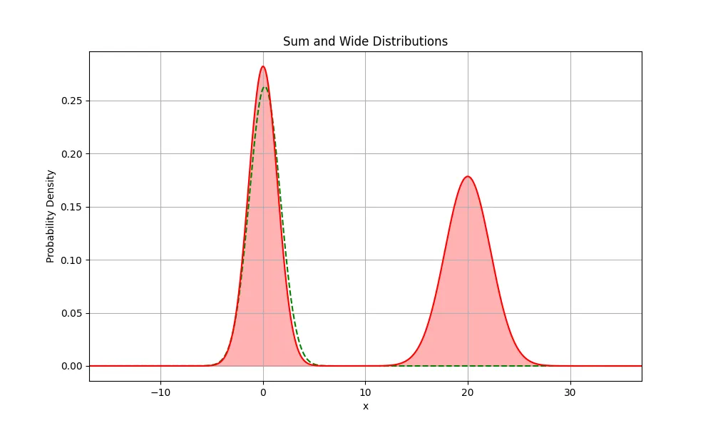
$Q(x)$ can be seen as a small deviation of $P(x)$. There may be one or more smaller modes across the models prediction distribution based on the type of task it completes.

If in this instance the KL divergence incentivises $Q(x)$ to not sit under the mode (basically the reference model’s exact distribution), the KL divergence will actually push the $Q(x)$ away from the reference model. In this use case this will introduce more variance and achieve the opposite of its goal.

How can we ensure then that in training objectives like this, we won't diverge away from our reference model too much?

The Backward KL Divergence

The backward KL divergence seeks to perform the exact same task as the Kullback-Leibler divergence, namely to give a measure for the amount one distribution "diverges" or moves away from another, but instead of calculating the divergence $K[P(x)||Q(x)], it instead calculates $K[Q(x)||P(x)].

The primary change here becomes that the weighting changes from being $P(x)$ to $Q(x)$.

Analysis of behaviour

Let's explore how the Backward KL Divergence behaves in each of the different possible locations of $Q(x)$. Since the $Q(x)$ is the factor that weighs the importance of the penalty in a region, the KL divergence maximises the amount of the $P(x)$ distribution that is captured in the area under $Q(x)$.

Far left or far right

At these positions, the KL divergence would be extremely high because the weighting of the divergence is most strongly influenced by the area under $Q(x)$ and the area under the curve in these regions is super low.

Immediate left or far right

At these positions, the KL divergence would be much lower because the area under $Q(x)$ is overlapping strongly to the available mode's, hence KL Divergence penalty is very low here while the weighting is maximally high.

Centre

At this position, the weighting will be highest in an area that does not have very much of the $P(x)$ region. The KL importance weighting of this region will thus be very high but will contain very little $P(x)$, making the KL penalty very high.

Analysis of behaviour

So out of the above scenarios, the most likely outcome will be that the $Q(x)$ distribution will simply stay as close to the original reference model's mode as possible. It won't be able to nudge away to move under another mode because it would need to push into a region of very high KL penalty first to do that.

In order to visualise how this might look in a real example, let's suppose we are at the language modelling head of some model and it is creating a distribution over the words it knows. This distribution tries to predict the most likely next word in the sentence.

In this scenario, there will be multiple words available that can be added to the sentence and still be valid but there will also be lots of words that are only slightly suitable. This means that the distribution will have a few peaks (modes) at some words while the other words will be very low or zero.

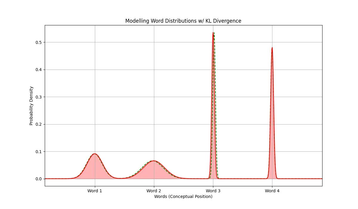
In this scenario, the KL divergence will try to minimise the divergence of $Q(x)$ under the word 3 and 4 modes with the highest importance. In our language model, this is exactly what we need as well.

#AI #Math #Reinforcement Learning